Static vs Dynamic libraries

Static Linking and Static Libraries:

====================================

Static Linking and Static Libraries is the result of the linker making copy of all used library functions to the executable file. Static Linking creates larger binary files, and need more space on disk and main memory. Examples of static libraries (libraries which are statically linked) are, .a files in Linux and .lib files in Windows.

Compile library files.

 gcc -c lib_mylib.c -o lib_mylib.o

Create static library. This step is to bundle multiple object files in one static library (see ar for details). The output of this step is static library.

 ar rcs lib_mylib.a lib_mylib.o 

Following are some important points about static libraries.
1. For a static library, the actual code is extracted from the library by the linker and used to build the final executable at the point you compile/build your application.

2. Each process gets its own copy of the code and data. Where as in case of dynamic libraries it is only code shared, data is specific to each process. For static libraries memory footprints are larger. For example, if all the window system tools were statically linked, several tens of megabytes of RAM would be wasted for a typical user, and the user would be slowed down by a lot of paging.

3. Since library code is connected at compile time, the final executable has no dependencies on the the library at run time i.e. no additional run-time loading costs, it means that you don’t need to carry along a copy of the library that is being used and you have everything under your control and there is no dependency.

4. In static libraries, once everything is bundled into your application, you don’t have to worry that the client will have the right library (and version) available on their system.

5. One drawback of static libraries is, for any change(up-gradation) in the static libraries, you have to recompile the main program every time.

6. One major advantage of static libraries being preferred even now “is speed”. There will be no dynamic querying of symbols in static libraries. Many production line software use static libraries even today.

 

 

Dynamic linking and Dynamic Libraries:

====================================

Dynamic linking and Dynamic Libraries Dynamic Linking doesn’t require the code to be copied, it is done by just placing name of the library in the binary file. The actual linking happens when the program is run, when both the binary file and the library are in memory. Examples of Dynamic libraries (libraries which are linked at run-time) are, .so in Linux and .dll in Windows.

[root@host ~]# gcc -Wall -fPIC -c add.c 
[root@host ~]# gcc -Wall -fPIC -c sub.c

[root@host ~]# gcc -shared -o libheymath.so add.o sub.o

 

Static Linking	Dynamic Linking
Static linking is the process of copying all library modules used in the program into the final executable image. This is performed by the linker and it is done as the last step of the compilation process. The linker combines library routines with the program code in order to resolve external references, and to generate an executable image suitable for loading into memory. When the program is loaded, the operating system places into memory a single file that contains the executable code and data. This statically linked file includes both the calling program and the called program.	In dynamic linking the names of the external libraries (shared libraries) are placed in the final executable file while the actual linking takes place at run time when both executable file and libraries are placed in the memory. Dynamic linking lets several programs use a single copy of an executable module.
Static linking is performed by programs called linkers as the last step in compiling a program. Linkers are also called link editors.	Dynamic linking is performed at run time by the operating system.
Statically linked files are significantly larger in size because external programs are built into the executable files.	In dynamic linking only one copy of shared library is kept in memory. This significantly reduces the size of executable programs, thereby saving memory and disk space.
In static linking if any of the external programs has changed then they have to be recompiled and re-linked again else the changes won’t reflect in existing executable file.	In dynamic linking this is not the case and individual shared modules can be updated and recompiled. This is one of the greatest advantages dynamic linking offers.
Statically linked program takes constant load time every time it is loaded into the memory for execution.	In dynamic linking load time might be reduced if the shared library code is already present in memory.
Programs that use statically-linked libraries are usually faster than those that use shared libraries.	Programs that use shared libraries are usually slower than those that use statically-linked libraries.
In statically-linked programs, all code is contained in a single executable module. Therefore, they never run into compatibility issues.	Dynamically linked programs are dependent on having a compatible library. If a library is changed (for example, a new compiler release may change a library), applications might have to be reworked to be made compatible with the new version of the library. If a library is removed from the system, programs using that library will no longer work.

Inline vs Macro in C

Inline:

• Is there a big difference between “regular” code and inline code?

Yes and no. No, because an inline function or method has exactly the same characteristics as a regular one, most important one being that they are both type safe. And yes, because the assembly code generated by the compiler will be different; with a regular function, each call will be translated into several steps: pushing parameters on the stack, making the jump to the function, popping the parameters, etc, whereas a call to an inline function will be replaced by its actual code, like a macro.

• Is inline code simply a “form” of macros?

No! A macro is simple text replacement, which can lead to severe errors. Consider the following code:

#define unsafe(i) ( (i) >= 0 ? (i) : -(i) )

[...]
unsafe(x++); // x is incremented twice!
unsafe(f()); // f() is called twice!
[...]

Using an inline function, you’re sure that parameters will be evaluated before the function is actually performed. They will also be type checked, and eventually converted to match the formal parameters types.

• What kind of tradeoff must be done when choosing to inline your code?

Normally, program execution should be faster when using inline functions, but with a bigger binary code. For more information, you should read GoTW#33.

 

========================================

Preprocessor macros are just substitution patterns applied to your code. They can be used almost anywhere in your code because they are replaced with their expansions before any compilation starts.

Inline functions are actual functions whose body is directly injected into their call site. They can only be used where a function call is appropriate.

Now, as far as using macros vs. inline functions in a function-like context, be advised that:

• Macros are not type safe, and can be expanded regardless of whether they are syntatically correct – the compile phase will report errors resulting from macro expansion problems.
• Macros can be used in context where you don’t expect, resulting in problems
• Macros are more flexible, in that they can expand other macros – whereas inline functions don’t necessarily do this.
• Macros can result in side effects because of their expansion, since the input expressions are copied wherever they appear in the pattern.
• Inline function are not always guaranteed to be inlined – some compilers only do this in release builds, or when they are specifically configured to do so. Also, in some cases inlining may not be possible.
• Inline functions can provide scope for variables (particularly static ones), preprocessor macros can only do this in code blocks {…}, and static variables will not behave exactly the same way.

 

Sample Program to Understand both:

#define square(x) x*x int main() {   int x = 36/square(6); // Expanded as 36/6*6   printf("%d", x);   return 0; } // Output: 36

If we use inline functions, we get the expected output. Also the program given in point 4 above can be corrected using inline functions.

inline int square(int x) { return x*x; } int main() {   int x = 36/square(6);   printf("%d", x);   return 0; } // Output: 1

Print Matrix diagonally

Print Matrix in Spiral Form……

#include <stdio.h>

#define R 3

#define C 6

 

void spiralPrint(int m, int n, int a[R][C])

{

    int i, k = 0, l = 0;

 

    /*  k - starting row index

        m - ending row index

        l - starting column index

        n - ending column index

        i - iterator

    */

 

    while (k < m && l < n)

    {

        /* Print the first row from the remaining rows */

        for (i = l; i < n; ++i)

        {

            printf("%d ", a[k][i]);

        }

        k++;

 

        /* Print the last column from the remaining columns */

        for (i = k; i < m; ++i)

        {

            printf("%d ", a[i][n-1]);

        }

        n--;

 

        /* Print the last row from the remaining rows */

        if ( k < m)

        {

            for (i = n-1; i >= l; --i)

            {

                printf("%d ", a[m-1][i]);

            }

            m--;

        }

 

        /* Print the first column from the remaining columns */

        if (l < n)

        {

            for (i = m-1; i >= k; --i)

            {

                printf("%d ", a[i][l]);

            }

            l++;    

        }        

    }

}

 

/* Driver program to test above functions */

int main()

{

    int a[R][C] = { {1,  2,  3,  4,  5,  6},

        {7,  8,  9,  10, 11, 12},

        {13, 14, 15, 16, 17, 18}

    };

 

    spiralPrint(R, C, a);

    return 0;

}

Packet Flow between Switches and Routers

Please go through following link,

https://www.practicalnetworking.net/series/packet-traveling/host-to-host-through-a-router/

 

Host to Host through a Router

This article is a part of a series on Packet Traveling — everything that happens in order to get a packet from here to there. Use the navigation boxes to view the rest of the articles.

 

Packet Traveling

• OSI Model
• Key Players
• Host to Host Communication
• Host to Host through a Switch
• Host to Host through a Router
• Packet Traveling – Series Finale

We’ve looked at what it takes for two hosts directly connected to each other to communicate. And we’ve looked at what it takes for a host to speak to another host through a switch. Now we add another network device as we look at what it takes for traffic to pass from host to host through a Router.

This article will be the practical application of everything that was discussed when we looked at a Router as a key player in Packet Traveling. It might be worth reviewing that section before proceeding.

We will start by looking at the two major Router Functions, then see them in action as we look at Router Operation.

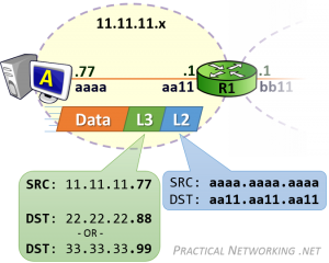
To discuss our way through these concepts, we will use the following image. We will focus on R1, and what is required for it to forward packets from Host A, to Host B and Host C.

For simplicity, the MAC addresses of each NIC will be abbreviated to just four hex digits.

Router Functions

Earlier we mentioned that a Router’s primary purpose is to facilitate communication between networks. As such, every router creates a boundary between two networks, and their main role is to forward packets from one network to the next.

Notice in the image above, we have R1 creating a boundary between the 11.11.11.x network and the 22.22.22.x network. And we have R2 creating a boundary between the 22.22.22.x and 33.33.33.x networks. Both of the routers have an interface in the 22.22.22.x network.

In order to forward packets between networks, a router must perform two functions: populate and maintain a Routing Table, and populate and maintain an ARP Table.

Populating a Routing Table

From the perspective of each Router, the Routing Table is the map of all networks in existence. The Routing Table starts empty, and is populated as the Router learns of new routes to each network.

There are multiple ways a Router can learn the routes to each network. We will discuss two of them in this section.

The simplest method is what is known as a Directly Connected route. Essentially, when a Router interface is configured with a particular IP address, the Router will know the Network to which it is directly attached.

For example, in the image above, R1’s left interface is configured with the IP address 11.11.11.1. This tells R1 the location of the 11.11.11.x network exists out its left interface. In the same way, R1 learns that the 22.22.22.x network is located on its right interface.

Of course, a Router can not be directly connected to every network. Notice in the image above, R1 is not connected to 33.33.33.x, but it is very likely it might have to one day forward a packet to that network. Therefore, there must exist another way of learning networks, beyond simply what the router is directly connected to.

That other way is known as a Static Route. A Static Route is a route which is manually configured by an administrator. It would be as if you explicitly told R1 that the 33.33.33.x network exists behind R2, and to get to it, R1 has to send packets to R2’s interface (configured with the IP address 22.22.22.2).

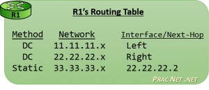
In the end, after R1 learned of the two Directly Connected routes, and after R1 was configured with the one Static Route, R1 would have a Routing Table that looked like this image.

The Routing Table is populated with many Routes. Each Route contains a mapping of Networks to Interfaces or Next-Hop addresses.

Every time a Router receives a packet, it will consult its Routing Table to determine how to forward the packet.

Again, the Routing Table is a map of every network that exists (from the perspective of each router). If a router receives a packet destined to a network it does not have a route for, then as far as that router is concerned, that network must not exist. Therefore, a router will discard a packet if its destination is in a network not in the Routing Table.

Finally, there is a third method for learning routes known as Dynamic Routing. This involves the routers detecting and speaking to one another automatically to inform each other of their known routes. There are various protocols that can be used for Dynamic Routing, each representing different strategies, but alas their intricacies fall outside the scope of this article series. They will undoubtedly become a subject for future articles.

That said, the Routing Table will tell the router which IP address to forward the packet to next. But as we learned earlier, packet delivery is always the job of Layer 2. And in order for the Router to create the L2 Header which will get the packet to the next L3 address, the Router must maintain an ARP Table.

Populating an ARP Table

The Address Resolution Protocol (ARP) is the bridge between Layer 3 and Layer 2. When provided with an IP address, ARP resolves the correlating MAC address. Devices employ ARP to populate an ARP Table, or sometimes called an ARP Cache, which is a mapping of IP address to MAC addresses.

A router will use its Routing Table to determine the next IP address which should receive a packet. If the Route indicates the destination exists on a directly connected network, then the “next IP address” is the Destination IP address of the packet – the final hop for that packet.

Either way, the Router will use a L2 header as the vessel to deliver the packet to the correct NIC.

Unlike the Routing Table, the ARP Table is populated ‘as needed’. Which means in the image above, R1 will not initiate an ARP Request for Host B’s MAC address until it has a packet which must be delivered to Host B.

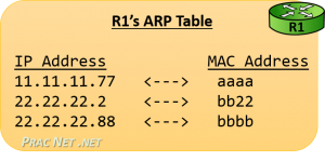
But as we discussed before, an ARP Table is simply a mapping of IP addresses to MAC addresses. When R1’s ARP Table will be fully populated, it will look like this image.

Once again, for simplicity, the images in this article are simply using four hex digits for the MAC addresses. In reality, a MAC address is 12 hex digits long. If its easier, you can simply repeat the four-digit hex MAC address three times, giving R2’s left interface a “real” MAC address of bb22.bb22.bb22.

 

Router Operation

With the understanding of how a Router populates its Routing Table and how a Router intends to populate its ARP Table, we can now look at how how these two tables are used practically for a Router to facilitate communication between networks.

In R1’s Routing Table above, you can see there are two type of routes: some that point to an Interface, and some that point to a Next-Hop IP address. We’ll frame our discussion around a Router’s operation around these two possibilities.

But first, we will discuss how Host A delivers the packet to its Default Gateway (R1). Then we will look at what R1 does with a packet sent from Host A to Host B, and then another packet that was sent from Host A to Host C.

 

Host A getting the Packet to R1

In both cases, Host A is communicating with two hosts on foreign networks. Therefore, Host A will need to get either packet to its default gateway — R1.

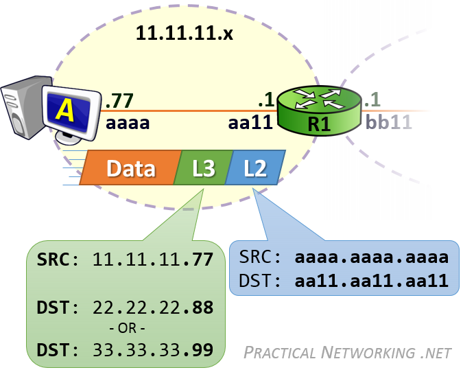
Host A will create the L3 header with a Source IP address of 11.11.11.77, and a Destination IP address of 22.22.22.88 (for Host B) or 33.33.33.99 (for Host C). This L3 header will serve the purpose of getting the data from ‘end to end’.

But that L3 header won’t be enough to deliver the packet to R1. Something else will have to be used.

Host A will then encapsulate the L3 header in a L2 header which will include a Source MAC address of aaaa.aaa.aaaa and a Destination MAC address of aa11.aa11.aa11 — the MAC address which identifies R1’s NIC. This L2 header will serve the purpose of delivering the packet across the first hop.

Host A will have already been configured with its Default Gateway’s IP address, and hopefully Host A will have already communicated with foreign hosts. As such, Host A more than likely already had an ARP Table entry with R1’s MAC address. Conversely, if this was Host A’s first communication with a foreign host, forming the L2 header would have been preceded with an ARP Request to discover R1’s MAC address.

At this point, R1 will have the packet. The Destination IP address of the packet will either be 22.22.22.88 for the communication sent to Host B, or 33.33.33.99 for the communication sent to Host C. Both of those destinations exist in R1’s Routing Table — the difference is one Route points to an Interface and the other Route points to a Next-Hop IP.

Routes pointing to an Interface

A Route in a Routing Table that points to an Interface was typically learned because the Router was Directly Connected to the network. If a packet’s Destination IP address is in a network which is directly connected to the router, the Router knows they are responsible for delivering the packet to its final hop.

The process is similar to what has been discussed before. The Router uses the L3 header information to determine where to send the packet next, then creates a L2 header to get it there. In this case, the next (and final) hop this packet must take is to the NIC on Host B.

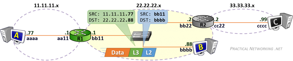
The L3 header will remain unchanged — it is identical to the L3 header created by Host A.

What is different, is the L2 header. Notice the Source MAC address is bb11.bb11.bb11 — R1’s right interface MAC address. The old L2 header which Host A had created to get the packet to R1 was stripped off, and a new L2 header was generated (by R1) to deliver it to the next NIC.

The Destination MAC address is, of course, bbbb.bbbb.bbbb — the MAC address for Host B.

 

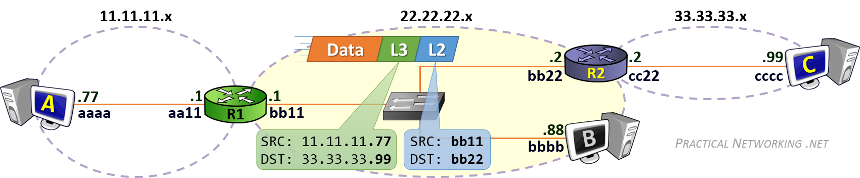
Routes pointing to a Next-Hop address

For the packet from Host A sent to Host C, the Destination IP address will be 33.33.33.99. When R1 consults its Routing Table, it will determine that the next-hop for the 33.33.33.x network exists at the IP address 22.22.22.2 — R2’s left interface IP address.

Effectively, this tells R1 to use a L2 header which will get the packet to R2 in order to continue forwarding this packet along its way.

Since the current “hop” is between R1 and R2, their MAC addresses will make up the Source and Destination MAC addresses:

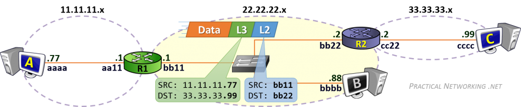
Again, the L3 header remains unchanged, it includes the same Source and Destination IP addresses initially set by Host A — these addresses represent the two “ends” of the communication. The L2 header, however, is completely regenerated at each hop.

Should R1 not have R2’s MAC address, it would simply initiate an ARP Request for the IP address in the route: 22.22.22.2. From then on, it will have no problems creating the proper L2 header which will get the packet from R1 to R2.

As the process continues, R2 will finally receive the packet, and then be faced with the same situation that R1 was in for the example above — deliver the packet to its final hop.

This process can be continued as needed. Had Host A been trying to speak to Host X which had 10 routers in the path, the process would have been identical. Each transit Router in the path would have a Route mapping Host X’s network to the next-hop IP in the path. Until the final router which would be directly connected to the network Host X resided in. And that final router would be responsible for delivering the packet to its final hop — Host X itself.

How Ping Works ?

Summary:

++++++++++

At this point, you should have a fairly complete understanding of the cycle of processing associated with ping.

Let me recapitulate the essential elements:

• As the ping program initializes, it opens a raw ICMP socket so that it can employ IP directly, circumvent-

ing

TCP and UDP

.

• Ping formats an ICMP type 8 message, an Echo Request, and sends it (using the “sendto” function) to

the designated target address. The system provides the IP header and the data link layer envelope.

¶s ICMP messages are received,

ping has the opportunity to examine each pack

et to pick out those

items that are of interest.

• The usual behavior is to siphon off ICMP type 0 messages, Echo Replies, which have an identification

field v

Link:  http://images.globalknowledge.com/wwwimages/whitepaperpdf/WP_Mays_Ping.pdf

alue that matches the program PID.

Understanding of extern storage class in C

Understanding “extern” keyword in C

2.8

I’m sure that this post will be as interesting and informative to C virgins (i.e. beginners) as it will be to those who are well versed in C. So let me start with saying that extern keyword applies to C variables (data objects) and C functions. Basically extern keyword extends the visibility of the C variables and C functions. Probably that’s is the reason why it was named as extern.

Though (almost) everyone knows the meaning of declaration and definition of a variable/function yet for the sake of completeness of this post, I would like to clarify them. Declaration of a variable/function simply declares that the variable/function exists somewhere in the program but the memory is not allocated for them. But the declaration of a variable/function serves an important role. And that is the type of the variable/function. Therefore, when a variable is declared, the program knows the data type of that variable. In case of function declaration, the program knows what are the arguments to that functions, their data types, the order of arguments and the return type of the function. So that’s all about declaration. Coming to the definition, when we define a variable/function, apart from the role of declaration, it also allocates memory for that variable/function. Therefore, we can think of definition as a super set of declaration. (or declaration as a subset of definition). From this explanation, it should be obvious that a variable/function can be declared any number of times but it can be defined only once. (Remember the basic principle that you can’t have two locations of the same variable/function). So that’s all about declaration and definition.

Now coming back to our main objective: Understanding “extern” keyword in C. I’ve explained the role of declaration/definition because it’s mandatory to understand them to understand the “extern” keyword. Let us first take the easy case. Use of extern with C functions. By default, the declaration and definition of a C function have “extern” prepended with them. It means even though we don’t use extern with the declaration/definition of C functions, it is present there. For example, when we write.

    int foo(int arg1, char arg2);

There’s an extern present in the beginning which is hidden and the compiler treats it as below.

    extern int foo(int arg1, char arg2);

Same is the case with the definition of a C function (Definition of a C function means writing the body of the function). Therefore whenever we define a C function, an extern is present there in the beginning of the function definition. Since the declaration can be done any number of times and definition can be done only once, we can notice that declaration of a function can be added in several C/H files or in a single C/H file several times. But we notice the actual definition of the function only once (i.e. in one file only). And as the extern extends the visibility to the whole program, the functions can be used (called) anywhere in any of the files of the whole program provided the declaration of the function is known. (By knowing the declaration of the function, C compiler knows that the definition of the function exists and it goes ahead to compile the program). So that’s all about extern with C functions.

Now let us the take the second and final case i.e. use of extern with C variables. I feel that it more interesting and information than the previous case where extern is present by default with C functions. So let me ask the question, how would you declare a C variable without defining it? Many of you would see it trivial but it’s important question to understand extern with C variables. The answer goes as follows.

    extern int var;

Here, an integer type variable called var has been declared (remember no definition i.e. no memory allocation for var so far). And we can do this declaration as many times as needed. (remember that declaration can be done any number of times) So far so good. 🙂

Now how would you define a variable. Now I agree that it is the most trivial question in programming and the answer is as follows.

    int var;

Here, an integer type variable called var has been declared as well as defined. (remember that definition is the super set of declaration). Here the memory for var is also allocated. Now here comes the surprise, when we declared/defined a C function, we saw that an extern was present by default. While defining a function, we can prepend it with extern without any issues. But it is not the case with C variables. If we put the presence of extern in variable as default then the memory for them will not be allocated ever, they will be declared only. Therefore, we put extern explicitly for C variables when we want to declare them without defining them. Also, as the extern extends the visibility to the whole program, by externing a variable we can use the variables anywhere in the program provided we know the declaration of them and the variable is defined somewhere.

Now let us try to understand extern with examples.

Example 1:

int var; int main(void) {    var = 10;    return 0; }

Analysis: This program is compiled successfully. Here var is defined (and declared implicitly) globally.

Example 2:

extern int var; int main(void) {   return 0; }

Analysis: This program is compiled successfully. Here var is declared only. Notice var is never used so no problems.

Example 3:

extern int var; int main(void) {  var = 10;  return 0; }

Analysis: This program throws error in compilation. Because var is declared but not defined anywhere. Essentially, the var isn’t allocated any memory. And the program is trying to change the value to 10 of a variable that doesn’t exist at all.

Example 4:

#include "somefile.h" extern int var; int main(void) {  var = 10;  return 0; }

Analysis: Supposing that somefile.h has the definition of var. This program will be compiled successfully.

Example 5:

extern int var = 0; int main(void) {  var = 10;  return 0; }

Analysis: Guess this program will work? Well, here comes another surprise from C standards. They say that..if a variable is only declared and an initializer is also provided with that declaration, then the memory for that variable will be allocated i.e. that variable will be considered as defined. Therefore, as per the C standard, this program will compile successfully and work.

So that was a preliminary look at “extern” keyword in C.

I’m sure that you want to have some take away from the reading of this post. And I would not disappoint you. 🙂
In short, we can say

1. Declaration can be done any number of times but definition only once.
2. “extern” keyword is used to extend the visibility of variables/functions().
3. Since functions are visible through out the program by default. The use of extern is not needed in function declaration/definition. Its use is redundant.
4. When extern is used with a variable, it’s only declared not defined.
5. As an exception, when an extern variable is declared with initialization, it is taken as definition of the variable as well.

 

__________ | __________

 

 

 

 

 

 

 

 

 

 

 

 

 

 

 

Algorithms

Compilation Stages in C

Compiling a C program:- Behind the Scenes

2.3

C is a high level language and it needs a compiler to convert it into an executable code so that the program can be run on our machine.

How do we compile and run a C program?

Below are the steps we use on an Ubuntu machine with gcc compiler.

• We first create a C program using an editor and save the file as filename.c

   $ vi filename.c

  The diagram on right shows a simple program to add two numbers.

• Then compile it using below command.

   $ gcc –Wall filename.c –o filename

  The option -Wall enables all compiler’s warning messages. This option is recommended to generate better code.
  The option -o is used to specify output file name. If we do not use this option, then an output file with name a.out is generated.

• After compilation executable is generated and we run the generated executable using below command.

   $ ./filename

What goes inside the compilation process?

Compiler converts a C program into an executable. There are four phases for a C program to become an executable:

1. Pre-processing
2. Compilation
3. Assembly
4. Linking

By executing below command, We get the all intermediate files in the current directory along with the executable.

 $gcc –Wall –save-temps filename.c –o filename

The following screenshot shows all generated intermediate files.

Let us one by one see what these intermediate files contain.

Pre-processingThis is the first phase through which source code is passed. This phase include:

• Removal of Comments
• Expansion of Macros
• Expansion of the included files.

The preprocessed output is stored in the filename.i. Let’s see what’s inside filename.i: using $vi filename.i

In the above output, source file is filled with lots and lots of info, but at the end our code is preserved.
Analysis:

• printf contains now a + b rather than add(a, b) that’s because macros have expanded.
• Comments are stripped off.
• #include<stdio.h> is missing instead we see lots of code. So header files has been expanded and included in our source file.

CompilingThe next step is to compile filename.i and produce an; intermediate compiled output file filename.s. This file is in assembly level instructions. Let’s see through this file using $vi filename.s

The snapshot shows that it is in assembly language, which assembler can understand.

AssemblyIn this phase the filename.s is taken as input and turned into filename.o by assembler. This file contain machine level instructions. At this phase, only existing code is converted into machine language, the function calls like printf() are not resolved. Let’s view this file using $vi filename.o

LinkingThis is the final phase in which all the linking of function calls with their definitions are done. Linker knows where all these functions are implemented. Linker does some extra work also, it adds some extra code to our program which is required when the program starts and ends. For example, there is a code which is required for setting up the environment like passing command line arguments. This task can be easily verified by using $size filename.o and $size filename. Through these commands, we know that how output file increases from an object file to an executable file. This is because of the extra code that linker adds with our program.

Phyton Tutorial

C Programming Videos

http://freevideolectures.com/Course/2519/C-Programming-and-Data-Structures